How to: Format Cells Using a Three-Color Scale
- 3 minutes to read
This example demonstrates how to apply a three-color scale conditional formatting rule.
- First of all, specify the minimum, midpoint and maximum thresholds of a range to which the rule will be applied. Threshold values are determined by the ConditionalFormattingValue object that can be accessed via the ConditionalFormattingCollection.CreateValue method. The type of the threshold value is specified by one of the ConditionalFormattingValueType enumeration values and can be a number, percent, formula, or percentile. Call the ConditionalFormattingCollection.CreateValue method with the ConditionalFormattingValueType.MinMax parameter to set the minimum and maximum thresholds to the lowest and highest values in a range of cells, respectively.
To apply a conditional formatting rule represented by the ColorScale3ConditionalFormatting object, access the collection of conditional formats from the Worksheet.ConditionalFormattings property and call the ConditionalFormattingCollection.AddColorScale3ConditionalFormatting method with the following parameters:
- A CellRange object that defines a range of cells to which the rule is applied.
- A minimum threshold specified by the ConditionalFormattingValue object.
- A color corresponding to the minimum value in a range of cells.
- A midpoint threshold specified by the ConditionalFormattingValue object.
- A color corresponding to the middle value in a range of cells.
- A maximum threshold specified by the ConditionalFormattingValue object.
- A color corresponding to the maximum value in a range of cells.
Note
Transparency is not supported in conditional formatting.
To remove the ColorScale3ConditionalFormatting object, use the ConditionalFormattingCollection.Remove, ConditionalFormattingCollection.RemoveAt or ConditionalFormattingCollection.Clear methods.
ConditionalFormattingCollection conditionalFormattings = worksheet.ConditionalFormattings;
// Set the minimum threshold to the lowest value in the range of cells using the MIN() formula.
ConditionalFormattingValue minPoint = conditionalFormattings.CreateValue(ConditionalFormattingValueType.Formula, "=MIN($C$2:$D$15)");
// Set the midpoint threshold to the 50th percentile.
ConditionalFormattingValue midPoint = conditionalFormattings.CreateValue(ConditionalFormattingValueType.Percentile, "50");
// Set the maximum threshold to the highest value in the range of cells using the MAX() formula.
ConditionalFormattingValue maxPoint = conditionalFormattings.CreateValue(ConditionalFormattingValueType.Number, "=MAX($C$2:$D$15)");
// Create the three-color scale rule to determine how values in cells C2 through D15 vary. Red represents the lower values, yellow represents the medium values and sky blue represents the higher values.
ColorScale3ConditionalFormatting cfRule = conditionalFormattings.AddColorScale3ConditionalFormatting(worksheet.Range["$C$2:$D$15"], minPoint, Color.Red, midPoint, Color.Yellow, maxPoint, Color.SkyBlue);
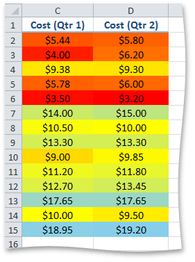
The image below shows the result (the workbook is opened in Microsoft® Excel®). Cost distribution is shown using a gradation of three colors. Red represents the lower values, yellow represents the medium values and sky blue represents the higher values.