Conditional Formatting
- 4 minutes to read
A Pivot dashboard item applies conditional formatting to cell values. You can calculate a format rule by measures placed in the Values section and dimensions placed in the Columns or Rows sections.
You can use hidden measures to specify a condition used to apply formatting to visible values.
Supported Format Rules
Format rules that can be applied to different data item types are as follows:
Data Type | Supported Format Conditions |
|---|---|
numeric | |
string | Value with the condition type set to Equal To, Not Equal To or Text that Contains |
date-time |
A Date Occurring for dimensions with the continuous date-time group interval |
Refer to the Conditional Formatting Basics topic for more information about format rule’s types.
Create and Edit a Format Rule
You can create and edit format rules in the following ways:
Click the Edit Rules button on the Home ribbon tab.
Click the measure/dimension menu button in the Data Item’s pane and select Add Format Rule/Edit Rules.
Refer to the following topic for information on how to create and edit format rules: Conditional Formatting in Windows Designer.
Pivot-Specific Format Condition Settings
You can configure and customize the format condition appearance settings.
Choose a predefined background color/font or click an empty square to add a new preset in the Appearance tab.
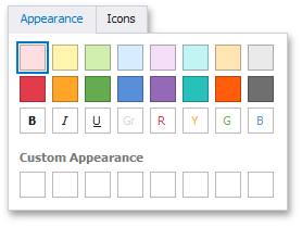
Add a predefined icon in the Icons tab.
The Appearance tab contains the following Pivot-specific settings:
| Option | Description |
|---|---|
| Enabled | Enables/ Disables the current format rule. |
| Intersection Mode | Specifies the level on which to apply conditional formatting to pivot cells. |
| Intersection Row/Column Dimension | Applies the format rule to the specified row/column dimension, if you select the Specific Level as the intersection mode. |
| Apply to Row/Column | Specifies whether to apply the formatting to the entire Pivot’s row/column. |
A Pivot item allows you to specify to which field intersection a format rule is applied.
| Intersection Level Mode | Description |
|---|---|
| Auto | Identifies the default level. For the Pivot dashboard item, Auto identifies the First Level. |
| First Level | The first level values are used to apply conditional formatting. |
| Last Level | The last level values are used to apply conditional formatting. |
| All Levels | All pivot data cells are used to apply conditional formatting. |
| Specific Level | The specified measures/dimensions are used to apply conditional formatting. |
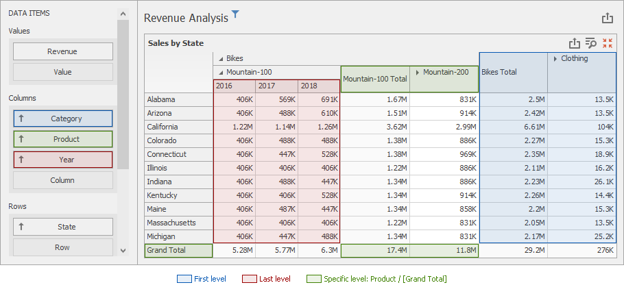
The image below displays different intersection levels with the applied conditional format rule:
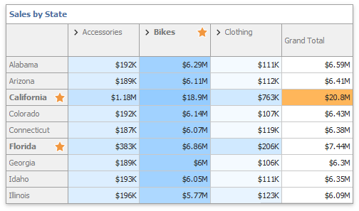
To apply a format rule to the row or column Grand Total, change the Intersection Level Mode to Specific level and set the [Grand Total] value as the intersection row/column dimension.
Note the following limitations:
- The dashboard cannot calculate conditional formatting in a Pivot for multiple levels of ranges with percentage values. In this case, the “All Levels” intersection mode is not available for a conditional formatting rule.
- The format condition dialog does not contain any Pivot-specific settings for a dimension from Columns and Rows.
Create a Format Rule in Code
Create a PivotItemFormatRule object and specify its settings to add a format rule:
- Create a condition (the FormatConditionBase descendant), specify its settings, and assign the resulting object to the DashboardItemFormatRule.Condition property.
- Assign a data item (measure/dimension) whose values are used to calculate the condition to the CellsItemFormatRule.DataItem property. Use the CellsItemFormatRule.DataItemApplyTo property to select measure/dimension values for which you want to apply a format rule. If this property is not specified, the control applies formatting to the CellsItemFormatRule.DataItem value.
- Use the PivotItemFormatRule.IntersectionLevelMode property to specify the intersection level. If the PivotItemFormatRule.IntersectionLevelMode property is set to FormatConditionIntersectionLevelMode.SpecificLevel, use the PivotItemFormatRule.Level property to set the intersection’s row and column fields.
- Add the created format rule to the GridDashboardItem.FormatRules collection.
Enable the CellsItemFormatRule.ApplyToRow/PivotItemFormatRule.ApplyToColumn properties to apply formatting to the entire pivot row/column.
You can use the DashboardItemFormatRule.Enabled property to disable the current format rule.
The following code snippet shows how to apply the Top-Bottom (FormatConditionTopBottom) format condition to highlight the three top values:
PivotItemFormatRule lastLevelRule = new PivotItemFormatRule(pivot.Values[0]);
FormatConditionRangeGradient rangeCondition =
    new FormatConditionRangeGradient(FormatConditionRangeGradientPredefinedType.WhiteGreen);
lastLevelRule.Condition = rangeCondition;
lastLevelRule.IntersectionLevelMode = FormatConditionIntersectionLevelMode.LastLevel;

PivotItemFormatRule topCategoryRule = new PivotItemFormatRule(pivot.Values[0]);
FormatConditionTopBottom topCondition = new FormatConditionTopBottom();
topCondition.TopBottom = DashboardFormatConditionTopBottomType.Top;
topCondition.RankType = DashboardFormatConditionValueType.Number;
topCondition.Rank = 3;
topCondition.StyleSettings = new IconSettings(FormatConditionIconType.RatingFullGrayStar);
topCategoryRule.Condition = topCondition;
topCategoryRule.IntersectionLevelMode = FormatConditionIntersectionLevelMode.SpecificLevel;
topCategoryRule.Level.Row = pivot.Rows[0];
topCategoryRule.DataItemApplyTo = pivot.Rows[0];

pivot.FormatRules.AddRange(lastLevelRule, topCategoryRule);
Tip
Refer to the Conditional Formatting section for more examples.