Tutorial 4 - Customize the Pivot Grid Appearance
- 4 minutes to read
The tutorial explains how to highlight key metrics, such as the products with the highest year-over-year sales growth, and how to customize the control’s appearance. In the previous tutorial, you added the Difference Variation by Year field that displays the percentage difference in sales between the previous and current years, and sorted products from the highest to lowest sales within categories according to total product sales. In this tutorial, you change the appearance of total and grand total cells and apply format rules to the Difference Variation by Year field.
Change the Pivot Grid Appearance
In this section, you will change the appearance of total and grand total cells. You will apply a lighter background color so that you can later emphasize other cells.
Click the Appearances page of the PivotGrid Designer. In the Appearances pane, select TotalCell and specify the BackColor property.

Select the “Azure” color.

Apply the same color to GrandTotalCell.
Apply Conditional Formatting
The Pivot Grid includes a Microsoft Excel-inspired conditional formatting feature that allows you to change the appearance of individual cells based on specific conditions. You can highlight important information, identify trends and exceptions, and compare data using the collection of format rules.
Highlight Highest Yearly Sales Increases
To highlight the highest percent increase in sales among products, you need to create a “Format only top or bottom ranked values” rule type and apply it to the target cells.
Open the PivotGrid Designer and go to the Format Rules page. Click Add Format Rule to create a new rule:

- Apply the following rule’s settings in the Properties pane:
Measure: pivotGridField5
Name: Products with the Highest Increase in Sales
Rule: Format only top or bottom ranked values
The
Ruleproperty’s value is displayed as FormatConditionRuleTopBottom.
Settings: Format cells by Row and Column field
Column: pivotGridField4
Row: pivotGridField1

The image below displays the Properties pane with the configured rule.

- Specify rule’s appearance and condition settings in the Rule pane:
Rank: 20
RankType: Percent
BackColor: 0, 192, 192

The image below displays the Rule pane with the configured appearance and condition settings.

When you run the application, the Pivot Grid highlights the top 20% of values in the Difference Variation by Year field (the cutoff value is 20).

Highlight Sales Decline Numbers
To highlight annual negative sales growth for categories, you need to create a “Format based on value” rule type and apply it to total cells.
Add one more rule in the Format Rules page.
- Apply the following rule settings in the Properties pane:
Measure: pivotGridField5
Name: Annual Negative Sales Growth
Rule: Format based on value
The
Ruleproperty’s value is displayed as FormatConditionRuleValue.
Settings: Format cells by Row and Column field
Column: pivotGridField4
Row: pivotGridField2
The image below displays the Properties pane with the configured rule.

- Specify rule’s appearance and condition settings in the Rule pane:
Condition: Less
Value1: 0
BackColor: 255, 128, 128

The image below displays the Rule pane with the configured appearance and condition settings.

When you run the application, the Pivot Grid highlights the negative difference in sales between product categories for different years.

Enable End-User Access to Conditional Formatting Rules
End users can manage the created rules in the UI. Set the PivotGridOptionsMenu.EnableFormatRulesMenu property to true to allow users to invoke the Conditional Formatting Rules Manager. To invoke this manager at runtime, right-click any Pivot Grid cell and select Manage Rules… from the Format Rules context menu.
The image below displays the invoked Conditional Formatting Rules Manager with the created rules.

Result
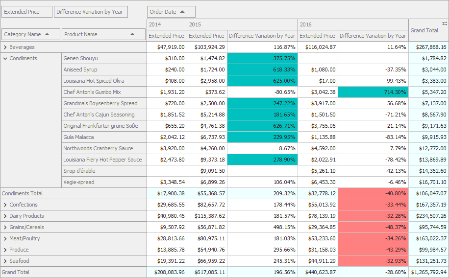
The image below shows the resulting Pivot Grid. You can compare multiple indicators according to displayed data:
- Product sales for several years.
- Contribution of each product to total sales.
- Percentage difference in sales between the previous and current years.
- Products with the highest increase in sales.
- Annual negative sales growth.
Related Documentation
The following help topics contain information about functionality used in the tutorial: