Conditional Formatting

• Oct 04, 2018
• 4 minutes to read

The Pivot dashboard item supports the conditional formatting feature that provides the capability to apply formatting to cells whose values meet the specified condition. This feature allows you to highlight specific cells or entire rows/columns using a predefined set of rules. To learn more about conditional formatting concepts common for all dashboard items, see the Conditional Formatting topic.

• Conditional Formatting Overview
• Create a Format Rule
• Edit a Format Rule
• Create a Format Rule in Code

Conditional Formatting Overview

The Pivot dashboard item allows you to use conditional formatting to measures placed in the Values section and dimensions placed in the Columns/Rows sections.

Note

Note that you can use hidden measures to specify a condition used to apply formatting to visible values.

New appearance settings are applied to pivot data cell or cells corresponding to column/row field values.

Create a Format Rule

To create a new format rule for the Pivot’s dimension/measure, do one of the following.

• Click the Options button next to the required measure/dimension, select Add Format Rule and choose the condition.
• Use the Edit Rules dialog.

Depending on the selected format condition, the dialog used to create a format rule for Pivot contains different settings. For instance, the image below displays the Greater Than dialog invoked for the measure.

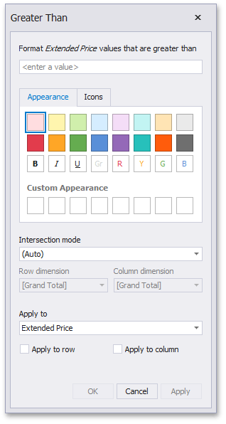
This dialog contains the following settings specific to Pivot.

• Intersection mode specifies the level on which to apply conditional formatting to pivot cells. The following levels are supported.

  1. Auto - Identifies the default level. For the Pivot dashboard item, Auto identifies the First Level.
  2. First Level - First level values are used to apply conditional formatting.
  3. Last Level - The last level values are used to apply conditional formatting.
  4. All Levels - All pivot data cells are used to apply conditional formatting.
  5. Specific Level - Values from the specific level are used to apply conditional formatting.
• If you specified the Intersection mode as Specific Level, use the Row dimension and Column dimension combo boxes to set the specific level.
• The Apply to row and Apply to column check boxes allow you to specify whether to apply the formatting to the entire pivot row/column.

Take note of the following behaviors specifics:

1. The dashboard does not provide the capability to calculate conditional formatting in the pivot grid for multiple levels for ranges with percentage values. In this case, the “All Levels” intersection mode is missing for a conditional formatting rule.
2. If you create a new format rule for a dimension from the Columns/Rows section, the corresponding format condition dialog would not contain any Pivot specific settings.

Edit a Format Rule

To edit format rules for the current Grid dashboard item, use the following options.

• Click the Edit Rules button in the Home ribbon tab or use corresponding item in the Pivot context menu.
• Click the menu button for the required data item and select Edit Rules.

Both these actions invoke the Edit Rules dialog containing existing format rules. To learn more, see Conditional Formatting.

Create a Format Rule in Code

The Pivot dashboard item allows you to apply conditional formatting to data cells or field value cells. The PivotDashboardItem.FormatRules property provides access to a collection of PivotItemFormatRule objects that are used to define formatting settings.

To add a new format rule, create the PivotItemFormatRule object and specify the following settings.

• Create a required condition (the FormatConditionBase descendant), specify its settings and assign the resulting object to the DashboardItemFormatRule.Condition property.
• Set a measure/dimension whose values are checked using the specified condition by specifying the CellsItemFormatRule.DataItem property. The CellsItemFormatRule.DataItemApplyTo property specifies the measure/dimension to whose values the formatting should be applied.
• Specify the intersection level used to apply formatting using the PivotItemFormatRule.IntersectionLevelMode property. If the PivotItemFormatRule.IntersectionLevelMode property is set to FormatConditionIntersectionLevelMode.SpecificLevel, specify the intersection level manually using the PivotItemFormatRule.Level property.
• Optionally, enable the CellsItemFormatRule.ApplyToRow/PivotItemFormatRule.ApplyToColumn flags to apply formatting to the entire pivot row/column.

Finally, add the created format rule to the GridDashboardItem.FormatRules collection. You can use the DashboardItemFormatRule.Enabled property to specify whether the current format rule is enabled.