How to: Format Top or Bottom Ranked Values
- 2 minutes to read
This example demonstrates how to apply a "top/bottom N" conditional formatting rule.
To create a new conditional formatting rule represented by the RankConditionalFormatting object, access the collection of conditional formats from the Worksheet.ConditionalFormattings property and call the ConditionalFormattingCollection.AddRankConditionalFormatting method. Pass the following parameters:
- A Range object that defines a range of cells to which the rule is applied.
- A condition specified by one of the ConditionalFormattingRankCondition enumeration values.
- A positive integer value representing the number or percentage of the rank value.
- Specify formatting options to be applied to cells if the condition is true, using the ISupportsFormatting.Formatting property of the RankConditionalFormatting object. Define the background and font colors, and set the outline borders.
To remove the RankConditionalFormatting object, use the ConditionalFormattingCollection.Remove, ConditionalFormattingCollection.RemoveAt or ConditionalFormattingCollection.Clear methods.
Note
A complete sample project is available at https://github.com/DevExpress-Examples/how-to-apply-conditional-formatting-to-a-range-of-cells-e4959
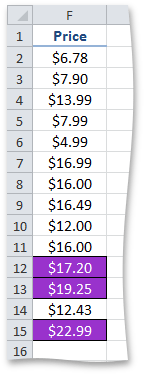
// Create the rule to identify top three values in cells F2 through F15.
RankConditionalFormatting cfRule = worksheet.ConditionalFormattings.AddRankConditionalFormatting(worksheet["$F$2:$F$15"], ConditionalFormattingRankCondition.TopByRank, 3);
// Specify formatting options to be applied to cells if the condition is true.
// Set the background color to dark orchid.
cfRule.Formatting.Fill.BackgroundColor = Color.DarkOrchid;
// Set the outline borders.
cfRule.Formatting.Borders.SetOutsideBorders(Color.Black, BorderLineStyle.Thin);
// Set the font color to white.
cfRule.Formatting.Font.Color = Color.White;
The image below shows the result (the workbook is opened in Microsoft® Excel®). The top three price values are highlighted.